Load libraries

rm(list = ls())
library(tidyverse)
library(lubridate)
library(ggplot2)
library(gganimate)
library(gridExtra)
library(scales)
theme_set(theme_light())

bird_counts <- readr::read_csv("https://raw.githubusercontent.com/rfordatascience/tidytuesday/master/data/2019/2019-06-18/bird_counts.csv")

bird_counts

## # A tibble: 18,706 x 6
##     year species    species_latin  how_many_counted total_hours how_many_counte…
##    <dbl> <chr>      <chr>                     <dbl>       <dbl>            <dbl>
##  1  1921 American … Botaurus lent…                0           8            0    
##  2  1921 American … Anas rubripes                 0           8            0    
##  3  1921 American … Fulica americ…                0           8            0    
##  4  1921 American … Corvus brachy…                0           8            0    
##  5  1921 American … Spinus tristis                0           8            0    
##  6  1921 American … Falco sparver…                0           8            0    
##  7  1921 American … Anthus rubesc…                0           8            0    
##  8  1921 American … Turdus migrat…                1           8            0.125
##  9  1921 American … Picoides dors…                0           8            0    
## 10  1921 American … Spizelloides …               12           8            1.5  
## # … with 18,696 more rows

bird_counts %>% 
  summary

##       year        species          species_latin      how_many_counted 
##  Min.   :1921   Length:18706       Length:18706       Min.   :    0.0  
##  1st Qu.:1947   Class :character   Class :character   1st Qu.:    0.0  
##  Median :1970   Mode  :character   Mode  :character   Median :    0.0  
##  Mean   :1970                                         Mean   :  193.5  
##  3rd Qu.:1994                                         3rd Qu.:    5.0  
##  Max.   :2017                                         Max.   :73000.0  
##                                                                        
##   total_hours    how_many_counted_by_hour
##  Min.   :  8.0   Min.   :  0.000         
##  1st Qu.:149.5   1st Qu.:  0.000         
##  Median :171.0   Median :  0.000         
##  Mean   :170.8   Mean   :  1.336         
##  3rd Qu.:203.8   3rd Qu.:  0.051         
##  Max.   :251.0   Max.   :439.024         
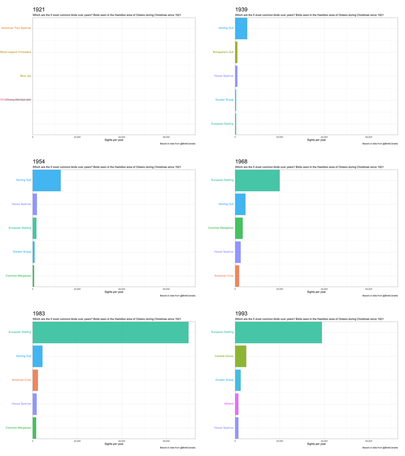
##  NA's   :3781    NA's   :3781

Which are the 5 most common birds over years?

bird_counts %>% 
  group_by(year) %>% 
  mutate(rank = min_rank(-how_many_counted) * 1) %>% 
  ungroup() %>% 
  filter(rank <= 5) %>% 
  ggplot(aes(rank, 
             group = species,
             fill = as.factor(species), 
             color = as.factor(species))) +
  geom_tile(aes(y = how_many_counted/2,
                height = how_many_counted,
                width = 0.9),
            alpha = 0.8, 
            color = NA) + 
  geom_text(aes(y = 0,
                label = paste(species, " ")),
            vjust = 0.2, 
            hjust = 1) + 
  coord_flip(clip = "off",
             expand = FALSE) + 
  scale_y_continuous(labels = scales::comma) + 
  scale_x_reverse() + 
  guides(color = FALSE,
         fill = FALSE) + 
  labs(title = '{closest_state}',
       subtitle = "Which are the 5 most common birds over years? Birds seen in the Hamilton area of Ontario during Christmas since 1921",
       caption = "Based on data from @BirdsCanada",
       x = "",
       y = "Sights per year") + 
  theme(plot.title = element_text(hjust = 0, size = 22),
        axis.ticks.y = element_blank(),
        axis.text.y = element_blank(),
        plot.margin = margin(1,1,1,4,"cm")) + 
  transition_states(year, transition_length = 4, state_length = 1) + 
  ease_aes('cubic-in-out') -> p

p %>% 
  animate(fps = 5,
          nframes = 200,
          duration = 30,
          width = 800,
          height = 600,
          renderer = gifski_renderer("../data/christmas_bird_counts/most_common.gif"))